Getting Started with RcppML

What Is RcppML?

RcppML decomposes a nonnegative matrix $A$ into low-rank factors $A \approx W \cdot \text{diag}(d) \cdot H$, where $W$ captures features, $H$ captures sample loadings, and $d$ gives per-factor scale.

Built on Rcpp and Eigen with OpenMP parallelism and optional CUDA GPU support, RcppML is designed for large sparse matrices common in genomics, recommender systems, and image analysis. Key capabilities include:

• NMF with coordinate-descent and Cholesky NNLS solvers
• SVD / PCA with optional non-negativity and L1 constraints
• Cross-validation via speckled holdout for automatic rank selection
• Distribution-aware losses: Gaussian, Poisson, Generalized Poisson, Negative Binomial, Gamma, Inverse Gaussian, Tweedie — plus zero-inflation
• Regularization: L1, L2, L21, angular, graph Laplacian, upper bounds
• Consensus clustering and divisive clustering (dclust)
• Composable factorization graphs via factor_net()
• StreamPress .spz format for out-of-core computation
• GPU acceleration via CUDA

Installation

Install from CRAN:

install.packages("RcppML")

Or install the development version:

remotes::install_github("zdebruine/RcppML")

For GPU support, see the GPU Acceleration vignette.

Quick NMF Demo

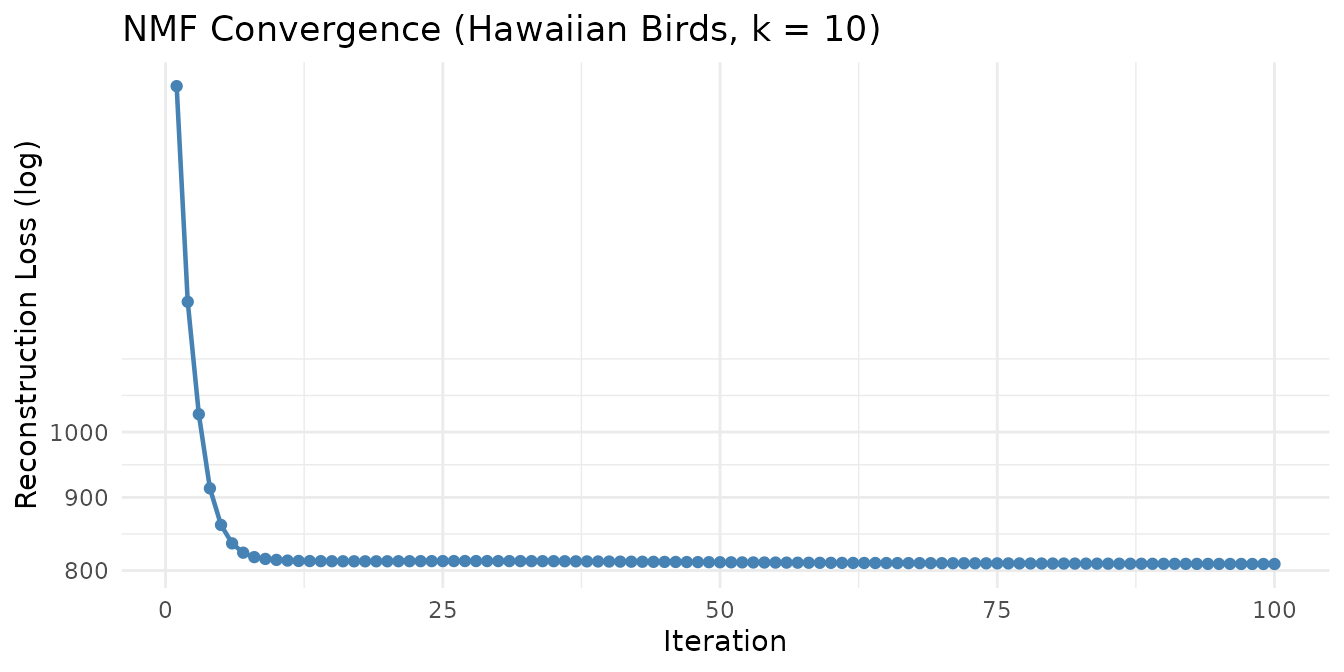
Factor the Hawaiian birds species-count matrix (183 species × 1,183 grid cells) into 10 components:

data(hawaiibirds)
model <- nmf(hawaiibirds, k = 10, seed = 42, tol = 1e-5, maxit = 100)

NMF model summary

Rows	Columns	Rank	Reconstruction MSE	Iterations	Runtime (sec)
183	1183	10	3.73e-03	100	0.28

Each of the 10 factors captures a distinct pattern of bird species co-occurrence across Hawaiian survey sites.

Quick SVD Demo

We can also decompose the same data with SVD, which captures directions of maximum variance rather than additive nonneg parts:

data(hawaiibirds)
sv <- svd(hawaiibirds, k = 10)

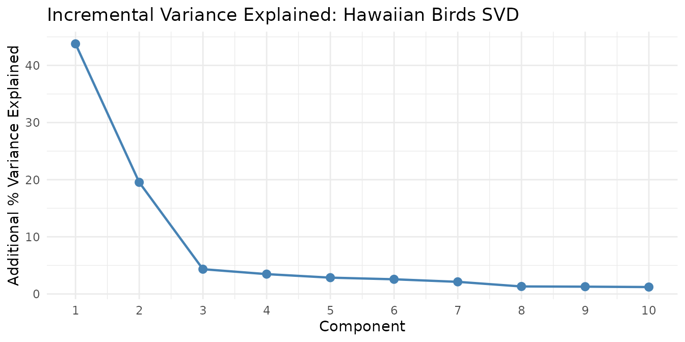
The first component captures the dominant species-composition gradient, and each subsequent component adds progressively less explanatory power — the hallmark of effective dimensionality reduction.

For PCA (centered and optionally scaled SVD), use the pca() convenience wrapper:

pc <- pca(hawaiibirds, k = 5, seed = 42)  # center = TRUE by default
# Equivalent to: svd(hawaiibirds, k = 5, center = TRUE)

PCA centers the data before decomposition, so the first component captures the dominant direction of variation rather than the overall mean level. Use scale = TRUE for data where features have different units or widely varying magnitude.

Quick Cross-Validation Demo

Use speckled holdout cross-validation to find the best rank for the AML data:

data(aml)
cv <- nmf(aml, k = c(2, 4, 6, 8, 10), test_fraction = 0.2, seed = 42)

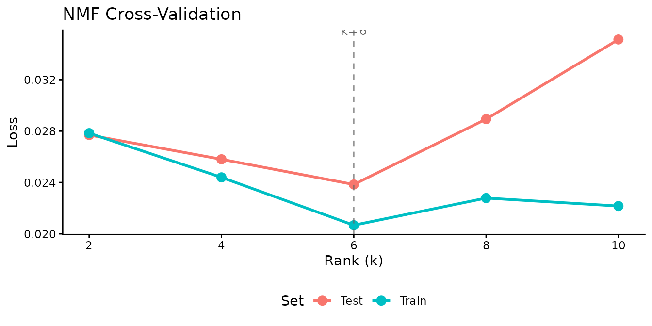
Training loss always decreases with rank, but test loss reveals where the model begins to overfit. The test-loss minimum identifies the optimal number of factors.

Built-in Datasets

RcppML ships seven datasets spanning diverse domains:

Shipped datasets

Dataset	Dimensions	Type	Domain
aml	824 × 135	Dense matrix	DNA methylation (AML)
golub	38 × 5,000	Sparse (dgCMatrix)	Gene expression (leukemia)
hawaiibirds	183 × 1,183	Sparse (dgCMatrix)	Bird species counts
movielens	3,867 × 610	Sparse (dgCMatrix)	Movie ratings
olivetti	400 × 4,096	Sparse (dgCMatrix)	Face images (Olivetti)
digits	1,797 × 64	Sparse (dgCMatrix)	Handwritten digit images
pbmc3k	13,714 × 2,638	SPZ raw bytes	Single-cell RNA-seq (PBMCs)

The pbmc3k dataset is stored as StreamPress-compressed raw bytes containing the full 13,714 genes × 2,638 cells from the 10x Genomics PBMC 3k dataset, with 9 Seurat-annotated cell types embedded as column metadata. Decompress it with st_read() and access annotations via st_read_var() — see the StreamPress vignette.

Where to Go Next

Core Techniques

• NMF Fundamentals — Solvers, diagonal scaling, convergence, and basic workflow
• SVD and PCA — Truncated SVD, PCA, non-negative and sparse variants
• Cross-Validation — Speckled holdout for automatic rank selection
• Statistical Distributions — Distribution-aware losses and zero-inflation handling
• Regularization and Constraints — L1, L2, L21, angular penalties, and upper bounds

Advanced Methods

• Clustering, Consensus, and Classification — Divisive clustering, consensus NMF, and sample classification
• Factorization Graphs — Multi-modal and guided factorization via factor_net()

Infrastructure

• StreamPress — High-performance sparse matrix compression and out-of-core NMF
• GPU Acceleration — CUDA-based GPU support for large-scale factorization