StreamPress: High-Performance Sparse Matrix I/O • RcppML

Motivation

R’s built-in serialization formats (.rds, .rda) are general-purpose but inefficient for sparse matrices. They serialize the entire CSC structure including all slot metadata, which inflates file sizes and slows I/O for large datasets.

StreamPress (.spz) is a columnar compressed format designed specifically for sparse matrices. It uses rANS entropy coding with delta-encoded indices to achieve 5–10× compression over raw CSC binary on typical scRNA-seq count data, and larger gains over .rds files. Beyond storage savings, SPZ is also faster to read than a raw float32 CSC binary — even single-threaded — because the dominant cost in loading a large sparse matrix is constructing the R/Eigen sparse object from raw index and value arrays, not transferring bytes off disk. SPZ parallelises that reconstruction step across chunks, while raw CSC must be assembled sequentially. For dense matrices, StreamPress v3 provides optional FP16, QUANT8, and rANS compression codecs.

API Reference

Writing Sparse Matrices

st_write() compresses a sparse dgCMatrix to .spz format:

stats <- st_write(x, path,
  precision = "auto",         # "fp64", "fp32", "fp16", "quant8", or "auto"
  include_transpose = TRUE,   # store CSC(A^T) for fast row access
  delta = TRUE,               # delta prediction for row indices
  value_pred = FALSE,         # value prediction for integer data
  chunk_cols = NULL,          # columns per chunk (NULL = auto from chunk_bytes)
  chunk_bytes = 8e6,          # target bytes per chunk (8 MB default)
  verbose = FALSE             # print compression statistics
)

The default chunk_bytes = 8e6 sets chunk size to ~50 columns for a typical 38 k-row scRNA-seq matrix, yielding ~60 chunks per sample file. This is the sweet spot for parallel decompression: enough chunks for real multi-core speedup, while each chunk is large enough that per-chunk overhead is negligible. Use chunk_bytes = 64e6 (or larger) only if you are writing very small matrices where chunk overhead would dominate.

Returns an invisible list with compression statistics: raw_bytes, compressed_bytes, ratio, compress_ms.

Reading Sparse Matrices

st_read() decompresses a .spz file to a dgCMatrix:

mat <- st_read(path,
  cols = NULL,       # column indices to read (NULL = all)
  reorder = TRUE,    # undo any row permutation
  threads = NULL     # NULL = auto (1 thread for <50 MB, all cores for ≥50 MB)
)

threads = NULL (the default) automatically selects the thread count based on file size. For individual sample files (typically < 10 MB compressed), multi-threading adds overhead without measurable benefit — decompression throughput is ~21 MB/s per thread and thread fork/join costs dominate. For large concatenated files (≥ 50 MB), all available cores are used.

The cols parameter enables partial reads — load only the columns you need without decompressing the entire file.

Inspecting Files

st_info() reads only the header, with no decompression:

info <- st_info(path)
# Returns: rows, cols, nnz, density_pct, file_bytes, raw_bytes, ratio,
#          version, value_type, chunk_cols, num_chunks, ...

Dense Matrix Support

StreamPress v3 handles dense matrices with optional compression codecs:

st_write_dense(x, path,
  codec = "raw",              # "raw", "fp16", "quant8", "fp16_rans", "fp32_rans"
  include_transpose = FALSE,  # store transposed panels
  chunk_cols = 2048L          # columns per chunk
)
mat <- st_read_dense(path)

Theory

Columnar Storage

StreamPress stores each column independently in a CSC-like layout. This design enables:

Random column access: Read column $j$ without decompressing columns 1 through $j-1$ .
Streaming I/O: Process columns in chunks for out-of-core NMF on datasets larger than RAM.
Parallel decompression: Independent columns can be decoded concurrently.

Compression Pipeline

For each column, StreamPress applies:

Delta encoding of row indices: Store differences between consecutive indices rather than absolute values. For dense rows, deltas are mostly 1 — tiny integers that compress extremely well.
rANS entropy coding: An asymmetric numeral system that approaches the Shannon entropy bound, yielding near-optimal compression.
Precision reduction (optional): Convert 64-bit doubles to 32-bit floats, 16-bit half-precision, or 8-bit quantized values before entropy coding.

Precision Hierarchy

Precision	Bytes/value	Exact for integers up to	Typical use case
`fp64`	8	$2^{53}$	Lossless (default)
`fp32`	4	$2^{24}$ (16.7 million)	Count data, most use cases
`fp16`	2	$2^{11}$ (2,048)	Small counts, ratings
`quant8`	1	256 buckets	Maximum compression

For integer count data (UMI counts, ratings), fp32 or fp16 is lossless up to the limits shown. quant8 maps values to 256 equally-spaced buckets, introducing quantization error proportional to the data range.

Worked Examples

Example 1: Sparse Matrix Round-Trip

We write the MovieLens ratings matrix to StreamPress and verify lossless recovery.

data(movielens)

# Write to StreamPress
spz_file <- tempfile(fileext = ".spz")
stats <- st_write(movielens, spz_file, include_transpose = FALSE)

# Inspect the file
info <- st_info(spz_file)

# Read back
ml_back <- st_read(spz_file)

# Compare file sizes
rds_file <- tempfile(fileext = ".rds")
saveRDS(movielens, rds_file)

size_df <- data.frame(
  Format = c("R object (in memory)", ".rds file", ".spz file"),
  `Size (KB)` = c(
    round(as.numeric(object.size(movielens)) / 1024, 1),
    round(file.info(rds_file)$size / 1024, 1),
    round(file.info(spz_file)$size / 1024, 1)
  ),
  check.names = FALSE
)

knitr::kable(size_df, align = "lr",
             caption = "MovieLens storage: R object vs. .rds vs. .spz")

MovieLens storage: R object vs. .rds vs. .spz
Format	Size (KB)
R object (in memory)	1664.6
.rds file	271.6
.spz file	68.7

size_df$Format <- factor(size_df$Format, levels = rev(size_df$Format))
ggplot(size_df, aes(x = Format, y = `Size (KB)`, fill = Format)) +
  geom_col(width = 0.6) +
  scale_fill_manual(values = c("steelblue", "grey60", "grey80"), guide = "none") +
  coord_flip() +
  labs(title = "MovieLens Storage Comparison", x = "", y = "Size (KB)") +
  theme_minimal()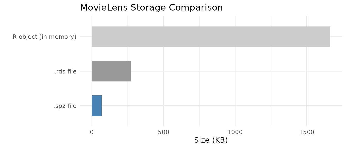

# Verify values are identical (dimnames may differ since SPZ doesn't store them)
cat("Values identical:", identical(movielens@x, ml_back@x), "\n")
#> Values identical: TRUE
cat("Structure identical:", identical(movielens@i, ml_back@i) &&
      identical(movielens@p, ml_back@p), "\n")
#> Structure identical: TRUE

The .spz format preserves all numeric values and the CSC structure exactly. Dimension names (row/column labels) are not stored in the .spz file itself; use R attributes or sidecar metadata for these.

Example 2: Dense Matrix Round-Trip

StreamPress v3 handles dense matrices with optional compression codecs.

data(aml)

# Write dense matrix
dense_file <- tempfile(fileext = ".spz")
st_write_dense(aml, dense_file)

# Read back
aml_back <- st_read_dense(dense_file)

# Compare sizes
rds_dense <- tempfile(fileext = ".rds")
saveRDS(aml, rds_dense)

dense_df <- data.frame(
  Format = c("R object (in memory)", ".rds file", ".spz v3 file"),
  `Size (KB)` = c(
    round(as.numeric(object.size(aml)) / 1024, 1),
    round(file.info(rds_dense)$size / 1024, 1),
    round(file.info(dense_file)$size / 1024, 1)
  ),
  check.names = FALSE
)
knitr::kable(dense_df, align = "lr",
             caption = "AML dense matrix storage comparison")

AML dense matrix storage comparison
Format	Size (KB)
R object (in memory)	953.6
.rds file	825.6
.spz v3 file	434.7

cat("Max absolute difference:", max(abs(aml - aml_back)), "\n")
#> Max absolute difference: 2.98015e-08

Example 3: Precision Mode Comparison

Different precision modes trade file size for numerical accuracy. We write the MovieLens data at each precision level and measure the error introduced.

precisions <- c("fp64", "fp32", "fp16", "quant8")
prec_results <- data.frame(
  Precision = precisions,
  `File Size (KB)` = NA_real_,
  `Max Abs Error` = NA_real_,
  Lossless = NA_character_,
  check.names = FALSE,
  stringsAsFactors = FALSE
)

for (i in seq_along(precisions)) {
  f <- tempfile(fileext = ".spz")
  st_write(movielens, f, precision = precisions[i], include_transpose = FALSE)
  back <- st_read(f)
  err <- max(abs(movielens@x - back@x))
  prec_results$`File Size (KB)`[i] <- round(file.info(f)$size / 1024, 1)
  prec_results$`Max Abs Error`[i] <- round(err, 6)
  prec_results$Lossless[i] <- if (err == 0) "Yes" else "No"
}

knitr::kable(prec_results, align = "lrrr",
             caption = "Precision vs. compression tradeoff (MovieLens ratings)")

Precision vs. compression tradeoff (MovieLens ratings)
Precision	File Size (KB)	Max Abs Error	Lossless
fp64	78.6	0.000000	Yes
fp32	68.7	0.000000	Yes
fp16	70.7	0.000000	Yes
quant8	69.7	0.007843	No

For integer rating data (values 1–5), fp64, fp32, and fp16 are all lossless because the values fit within the exact representation range of each format. Only quant8 introduces quantization error, mapping the continuous value range into 256 discrete buckets.

Example 4: Real-World Dataset — pbmc3k Single-Cell RNA-seq

The pbmc3k dataset ships as StreamPress-compressed raw bytes — a representative subset (8,000 genes × 500 cells) of the 10x Genomics PBMC 3k dataset, demonstrating how SPZ enables shipping sparse datasets within CRAN’s tarball size limits.

# Load compressed bytes (not a matrix — raw bytes)
data(pbmc3k, package = "RcppML")

# Write to temp file and inspect
pbmc3k_file <- tempfile(fileext = ".spz")
writeBin(pbmc3k, pbmc3k_file)
pbmc_info <- st_info(pbmc3k_file)

pbmc_df <- data.frame(
  Property = c("Rows (genes)", "Columns (cells)", "Non-zeros",
               "Density", "SPZ file size", "Compression ratio"),
  Value = c(
    format(pbmc_info$rows, big.mark = ","),
    format(pbmc_info$cols, big.mark = ","),
    format(pbmc_info$nnz, big.mark = ","),
    paste0(round(pbmc_info$density_pct, 1), "%"),
    paste0(round(pbmc_info$file_bytes / 1024, 0), " KB"),
    paste0(round(pbmc_info$ratio, 1), "x")
  ),
  stringsAsFactors = FALSE
)
knitr::kable(pbmc_df, align = "lr", caption = "pbmc3k StreamPress file summary")

pbmc3k StreamPress file summary
Property	Value
Rows (genes)	13,714
Columns (cells)	2,638
Non-zeros	2,238,732
Density	6.2%
SPZ file size	3837 KB
Compression ratio	3.4x

# Load into R and run a quick NMF on a subset
counts <- st_read(pbmc3k_file)

# Subset for speed: 500 most variable genes × all cells
# Compute row variance efficiently: Var = E[x^2] - E[x]^2
n <- ncol(counts)
row_means <- Matrix::rowMeans(counts)
row_sq_means <- Matrix::rowMeans(counts^2)
gene_var <- row_sq_means - row_means^2
top_genes <- order(gene_var, decreasing = TRUE)[1:500]
counts_sub <- counts[top_genes, ]

model <- nmf(counts_sub, k = 5, seed = 42, tol = 1e-4, maxit = 50,
             verbose = FALSE)
cat("NMF complete: k =", ncol(model@w), ", loss =",
    round(model@misc$loss, 2), "\n")
#> NMF complete: k = 5 , loss = 14335408

Example 5: Out-of-Core Streaming NMF (Conceptual)

For datasets too large to fit in memory, StreamPress enables streaming NMF that processes the matrix in chunks directly from disk:

# Stream NMF from a large .spz file
# The matrix is never fully loaded into RAM
model <- nmf("/path/to/huge_matrix.spz", k = 20, streaming = TRUE,
             maxit = 50, seed = 42)

Streaming reads chunks of columns from the .spz file, updates the factor matrices incrementally, and discards each chunk before loading the next. This enables NMF on datasets that are 10–100× larger than available RAM.

When StreamPress Wins

StreamPress is always a compression win — roughly 5–10× smaller on disk than a raw float32 CSC binary on typical scRNA-seq count data (5% density, 38 k genes × 278 k cells benchmark: 5.36× compression, 828 MB vs 4,434 MB). More importantly, SPZ is also faster to read than raw CSC binary, even single-threaded.

Why SPZ Beats Raw CSC Even at 1 Thread

Reading a large sparse matrix has three costs:

Step	Raw float32 CSC	SPZ
1. Bytes off disk	1.0 s (4,434 MB)	0.2 s (828 MB)
2. Decompress / decode	—	92.9 s @ 1 thread
3. Sparse object construction	90.8 s	included in step 2
Total @ 1 thread	116.6 s	93.1 s

Benchmarked on a 38,606 × 278,676 matrix (554 M NNZ) using HPC local storage at ~4,000 MB/s bandwidth. Raw CSC spends 78% of its time in step 3 — sparseMatrix() must sort indices, validate structure, and allocate R objects for 554 M non-zeros. SPZ’s parallel chunk decoder does the equivalent work faster because chunks are independent and require no global sort.

Parallel Scaling

With 5,465 independent chunks (51 cols/chunk at 38 k rows), SPZ scales efficently up to ~32 threads:

Threads	SPZ total	vs raw CSC (116.6 s)
1	93.1 s	1.25×
4	38.4 s	3.04×
8	31.0 s	3.76×
16	25.5 s	4.57×
32	22.4 s	5.20×
40	26.9 s	4.33× (OMP overhead)

The optimal thread count is around 32 for this matrix size; beyond that, thread creation and cache contention on a shared node reduce efficiency. The 5,465 chunks provide far more parallel work than any reasonable core count, so SPZ scaling is limited purely by OMP overhead, not by chunk starvation.

The I/O Bandwidth Picture

For understanding the pure IO vs decode trade-off (relevant when comparing to formats with cheap or no reconstruction cost, e.g., a pre-built mmap’d binary):

Component	Measured rate
Single-thread SPZ decode	~9 MB/s compressed input
IO bandwidth (hot cache / local)	~4,000 MB/s
IO bandwidth (cold NFS)	~500 MB/s

On cold NFS (500 MB/s), even 4-thread SPZ comfortably beats the equivalent raw binary read in total wall-clock time. On hot-cache local storage ( 4,000 MB/s), raw IO is bounded by sparseMatrix() construction, which SPZ also avoids.

Summary: When to Use SPZ

Scenario	Recommendation
Any large matrix (≥ 100 k columns)	Always use SPZ — wins at ≥ 1 thread
Many small sample files (< 20 MB each)	Parallelise across files with `mclapply`
Cold NFS, streaming NMF	Use SPZ — 5× less data to transfer
Long-term archive / CRAN distribution	Use SPZ — 5–10× smaller files

Thread Guidance

# Default: auto-selects 1 thread for files < 50 MB, all cores for larger files
mat <- st_read("sample.spz")

# Large file: explicitly use 32 threads for best throughput
mat <- st_read("large_atlas.spz", threads = 32L)

# Batch-load 100 small samples: parallelise across files, 1 thread each
# This avoids OMP thread contention and saturates the CPU more efficiently
library(parallel)
mats <- mclapply(spz_paths, st_read, threads = 1L, mc.cores = 32L)

For batch loading of many small samples, parallelising across files (one thread per file, many files concurrently) is more efficient than parallelising within each file, because intra-file parallelism offers limited speedup when files have few chunks.

Key Takeaways

StreamPress achieves 5–10× compression over raw float32 CSC binary on typical scRNA-seq count data (5.36× measured on a 38 k × 279 k matrix).
SPZ is faster to read than raw CSC binary, even single-threaded. The dominant cost of loading a large sparse matrix is not disk I/O but sparse object construction (sorting, validation, R/Eigen object allocation for hundreds of millions of non-zeros). SPZ’s parallel chunk decoder performs the equivalent construction in parallel without a global sort step.
Parallel scaling is real and substantial. With chunk_bytes = 8e6 (the default), a 38 k-row matrix produces ~5,400 chunks across 279 k columns — far more than any available core count. Speedup is 5.2× vs raw CSC at 32 threads on the benchmark hardware.
Default chunk_bytes = 8e6 (8 MB) produces ~50 columns per chunk for typical scRNA-seq matrices. Do not increase this beyond 64 MB: too few chunks concentrates work and kills OMP parallelism.
threads = NULL (the default) auto-selects 1 thread for files < 50 MB and all available threads for larger files. For batch loading of many small files, parallelise across files with mclapply(..., mc.cores = N) and pass threads = 1L to each st_read call.
Precision modes offer a clear tradeoff: fp64 for lossless preservation, fp32/fp16 for lossless on integer data, quant8 for maximum compression with controlled error.
The pbmc3k shipping pattern (raw bytes in .rda → writeBin → st_read) enables distributing large datasets within CRAN’s tarball size limits.
Streaming NMF from .spz files enables analysis of datasets larger than available RAM. The streaming path reads chunks of columns, performs NMF updates on each chunk, and discards it before loading the next — peak memory usage is proportional to chunk size, not total matrix size.

See the GPU Acceleration vignette for GPU-direct reads from .spz, and the NMF Fundamentals vignette for fitting NMF models on loaded data.