Non-negative matrix factorization

High-performance NMF of the form $A = wdh$ for large dense or sparse matrices. Supports single-rank fitting or cross-validation across multiple ranks. Returns an nmf object or nmfCrossValidate data.frame.

Usage

nmf(
  data,
  k,
  tol = 1e-04,
  maxit = 100,
  L1 = c(0, 0),
  L2 = c(0, 0),
  seed = NULL,
  mask = NULL,
  loss = c("mse", "gp", "nb", "gamma", "inverse_gaussian", "tweedie"),
  nonneg = c(TRUE, TRUE),
  test_fraction = 0,
  verbose = FALSE,
  projective = FALSE,
  symmetric = FALSE,
  zi = c("none", "row", "col"),
  robust = FALSE,
  ...
)

Arguments

data: dense or sparse matrix of features in rows and samples in columns. Prefer matrix or Matrix::dgCMatrix, respectively. Also accepts a file path (character string) which will be auto-loaded based on extension.
k: rank (integer), vector of ranks for cross-validation, or "auto" for automatic rank determination.
tol: tolerance of the fit (default 1e-4)
maxit: maximum number of fitting iterations (default 100)
L1: LASSO penalties in the range (0, 1], single value or array of length two for c(w, h)
L2: Ridge penalties greater than zero, single value or array of length two for c(w, h)
seed: initialization control. Accepts: NULL for random init, an integer for reproducible random init, a matrix (m x k) for custom W initialization, a list of matrices for multi-init, or a string: "lanczos", "irlba", "randomized", or "svd" (auto-select) for SVD-based initialization.
mask: missing data mask. Accepts: NULL (no masking), "zeros" (mask zeros), "NA" (mask NAs), a dgCMatrix/matrix (custom mask), or list("zeros", <matrix>) to mask zeros and use a custom mask simultaneously.
loss: loss function: "mse" (default), "gp", "nb", "gamma", "inverse_gaussian", or "tweedie". For robust loss (Huber/MAE), use the robust parameter instead.
nonneg: logical vector of length 2 for c(w, h) specifying non-negativity constraints (default c(TRUE, TRUE)).
test_fraction: fraction of entries to hold out for cross-validation (default 0 = disabled).
verbose: print progress information during fitting (default FALSE)
projective: if TRUE, use projective NMF (default FALSE).
symmetric: if TRUE, use symmetric NMF where H = W^T (default FALSE).
zi: zero-inflation mode: "none" (default), "row", or "col". Requires loss="gp" or loss="nb".
robust: robustness control. FALSE (default), TRUE (Huber delta=1.345), "mae" (near-MAE via very small Huber delta), or a positive numeric Huber delta. Huber loss is quadratic for small residuals and linear for large ones, controlled by delta. TRUE (delta=1.345) provides moderate outlier robustness. A large delta (e.g. 100) approaches standard MSE; a small delta (e.g. 0.01) approaches MAE. "mae" is shorthand for delta=1e-4 (effectively L1 loss).
...: advanced parameters. See Advanced Parameters section.

Value

When k is a single integer: an S4 object of class nmf with slots:

w: feature factor matrix, m x k
d: scaling diagonal vector of length k (descending order after sorting)
h: sample factor matrix, k x n
misc: list containing tol (final tolerance), iter (iteration count), loss (final loss value), loss_type (loss function used), and runtime (seconds).

When k is a vector: a data.frame of class nmfCrossValidate with columns k, rep, train_loss, test_loss, and best_iter.

Details

This fast NMF implementation decomposes a matrix $A$ into lower-rank non-negative matrices $w$ and $h$, with columns of $w$ and rows of $h$ scaled to sum to 1 via multiplication by a diagonal, $d$: $$A = wdh$$

The scaling diagonal ensures convex L1 regularization, consistent factor scalings regardless of random initialization, and model symmetry in factorizations of symmetric matrices.

The factorization model is randomly initialized. $w$ and $h$ are updated by alternating least squares.

RcppML achieves high performance using the Eigen C++ linear algebra library, OpenMP parallelization, a dedicated Rcpp sparse matrix class, and fast sequential coordinate descent non-negative least squares initialized by Cholesky least squares solutions.

Sparse optimization is automatically applied if the input matrix A is a sparse matrix (i.e. Matrix::dgCMatrix). There are also specialized back-ends for symmetric, rank-1, and rank-2 factorizations.

L1 penalization can be used for increasing the sparsity of factors and assisting interpretability. Penalty values should range from 0 to 1, where 1 gives complete sparsity.

Set options(RcppML.verbose = TRUE) to print model tolerances to the console after each iteration.

Parallelization is applied with OpenMP using the number of threads in getOption("RcppML.threads") and set by option(RcppML.threads = 0), for example. 0 corresponds to all threads, let OpenMP decide.

Cross-Validation

When k is a vector, the function performs cross-validation to find the optimal rank:

A fraction (test_fraction) of entries are held out for validation
Models are fit for each rank in k using only training data
Test loss is computed on held-out entries
Returns a data.frame with k, rep, train_mse, test_mse, and best_iter for each rank/replicate
Use plot() on the result to visualize loss vs rank

Loss Functions

The loss parameter controls the objective function:

"mse": Mean Squared Error (default). Standard Frobenius norm minimization.
"gp": Generalized Poisson. For overdispersed count data (e.g., scRNA-seq). Use dispersion to control per-row or global overdispersion estimation. With dispersion="none", equivalent to KL divergence (Poisson model).
"nb": Negative Binomial. Quadratic variance-mean relationship. Standard for scRNA-seq data with overdispersion. Size parameter (r) estimated per-row or globally.
"gamma": Gamma distribution. Variance proportional to mu^2. For positive continuous data. Dispersion (phi) estimated via MoM Pearson estimator.
"inverse_gaussian": Inverse Gaussian. Variance proportional to mu^3. For positive continuous data with heavy right tails.
"tweedie": Tweedie distribution. Variance proportional to mu^p where p is set via tweedie_power (default 1.5). Interpolates between Poisson (p=1), Gamma (p=2), and Inverse Gaussian (p=3).

For robust fitting (equivalent to Huber or MAE loss), use the robust parameter instead of a separate loss function. Setting robust = TRUE applies Huber-weighted IRLS with delta=1.345; robust = "mae" approximates mean absolute error.

Non-MSE losses use Iteratively Reweighted Least Squares (IRLS) which may be slower but provides better fits for count data (GP, NB) and positive continuous data (Gamma, Inverse Gaussian).

Advanced Parameters (via `...`)

The following parameters can be passed via ...:

Regularization:

L21: Group sparsity penalty, single value or c(w, h) (default c(0,0))
angular: Angular decorrelation penalty, c(w, h) (default c(0,0))
upper_bound: Box constraint on factors, c(w, h) (default c(0,0) = no bound)
graph_W, graph_H: Sparse graph Laplacian matrices for feature/sample regularization
graph_lambda: Graph regularization strength, c(w, h) (default c(0,0))
target_H: Target matrix (k x n) for H-side regularization. Steers H toward a desired structure during fitting. See compute_target.
target_lambda: Target regularization strength, single value or c(w, h) (default 0). Positive values attract H toward the target (label enrichment); negative values use PROJ_ADV eigenvalue-projected adversarial removal to suppress target-correlated structure (batch removal). See vignette("guided-nmf") for details.

Distribution Tuning:

dispersion: Dispersion mode for GP loss: "per_row", "per_col", "global", "none"
theta_init, theta_max, theta_min: GP theta bounds
nb_size_init, nb_size_max, nb_size_min: NB dispersion bounds
gamma_phi_init, gamma_phi_max, gamma_phi_min: Gamma/IG dispersion bounds
tweedie_power: Tweedie variance power (default 1.5)
irls_max_iter, irls_tol: IRLS convergence parameters

Zero-Inflation:

zi_em_iters: EM iterations per NMF step (default 1)

Solver:

solver: NNLS solver: "auto", "cholesky", "cd"
cd_tol: CD convergence tolerance (default 1e-8)
cd_maxit: CD max iterations (default 100)
h_init: Custom initial H matrix

Cross-Validation:

cv_seed: Separate seed(s) for CV holdout pattern
patience: Early stopping patience (default 5)
cv_k_range: Auto-rank search range (default c(2, 50))
track_train_loss: Track training loss in CV (default TRUE)

Resources & Output:

threads: OpenMP threads (default 0 = all)
resource: Compute backend: "auto", "cpu", "gpu"
norm: Factor normalization: "L1", "L2", "none"
sort_model: Sort factors by diagonal (default TRUE)

Streaming:

streaming: SPZ streaming mode: "auto", TRUE, FALSE
panel_cols: Panel size for streaming (default 0 = auto)
dispatch: StreamPress dispatch override

Callbacks:

on_iteration: Per-iteration callback function
profile: Enable timing profiling (default FALSE)

Compute Resources (CPU vs GPU)

By default (resource = "auto"), RcppML auto-detects available hardware. All features are fully supported on CPU (the default backend). GPU acceleration (when compiled with CUDA support) accelerates sparse and dense NMF. GPU is experimental and falls back to CPU automatically if unavailable.

Methods

S4 methods available for the nmf class:

predict: project an NMF model (or partial model) onto new samples
evaluate: calculate mean squared error loss of an NMF model
summary: data.frame giving fractional, total, or mean representation of factors in samples or features grouped by some criteria
align: find an ordering of factors in one nmf model that best matches those in another nmf model
prod: compute the dense approximation of input data
sparsity: compute the sparsity of each factor in $w$ and $h$
subset: subset, reorder, select, or extract factors (same as [)
generics such as dim, dimnames, t, show, head

References

DeBruine, ZJ, Melcher, K, and Triche, TJ. (2021). "High-performance non-negative matrix factorization for large single-cell data." BioRXiv.

Author

Zach DeBruine

Examples

# \donttest{
# basic NMF
model <- nmf(Matrix::rsparsematrix(1000, 100, 0.1), k = 10)

# cross-validation to find optimal rank
sim <- simulateNMF(200, 80, k = 5, noise = 3.0, seed = 42)
cv <- nmf(sim$A, k = 2:10, test_fraction = 0.05, cv_seed = 1:3,
          tol = 1e-5, maxit = 200)
plot(cv)

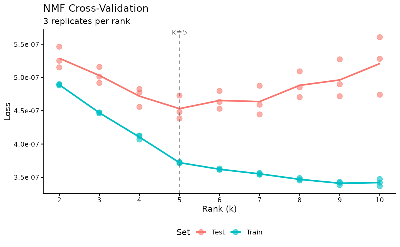optimal_k <- cv$k[which.min(cv$test_mse)]

# fit final model with optimal rank
model <- nmf(sim$A, optimal_k)
# }