GPU-Accelerated Computing

Motivation

At scale, dimensionality reduction is bottlenecked by dense linear algebra. Each NMF iteration computes Gram matrices ($H H^T$, $W^T W$) and right-hand-side products ($A H^T$, $W^T A$) — operations that map directly onto GPU hardware where thousands of cores execute matrix multiplies in parallel. RcppML’s GPU backend uses NVIDIA CUDA with cuBLAS and cuSPARSE to accelerate these operations, achieving 10–40× speedups on real single-cell datasets even against a fully-utilized 56-thread CPU.

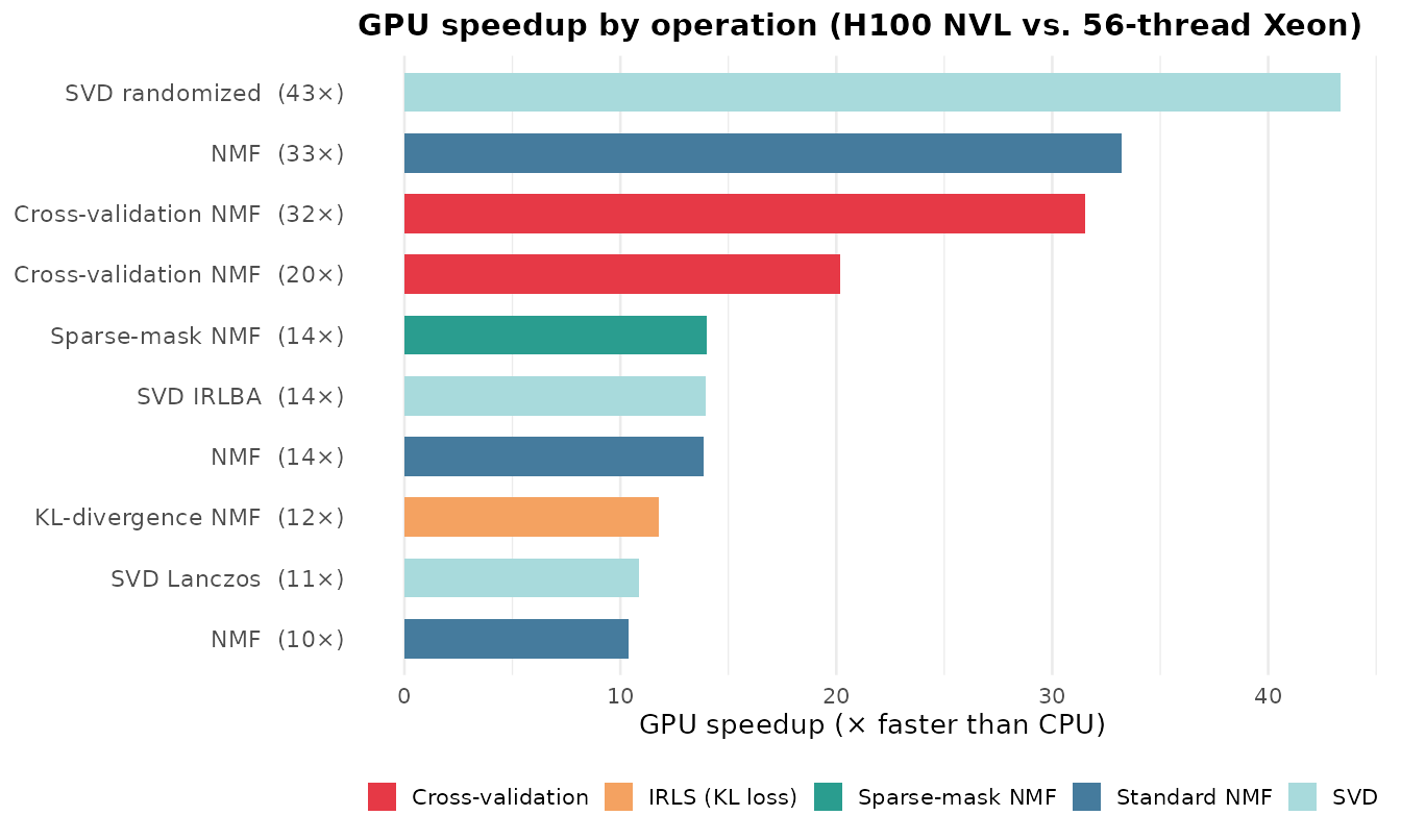
The GPU advantage is not uniform across operations. Standard NMF already benefits significantly, but cross-validation and SVD randomized show the largest gains because these modes perform dense BLAS work (Gram matrix corrections, block matrix multiplies) that maps directly onto GPU hardware. The GPU is optional — all code falls back to CPU transparently when CUDA is unavailable.

Quick Start

library(RcppML)

# Check GPU availability
gpu_available()
#> [1] TRUE
gpu_info()
#>   device              name total_mb free_mb
#> 1      0  NVIDIA H100 NVL    95830   93500

# NMF with GPU — same API, add resource = "gpu"
model <- nmf(A, k = 20, resource = "gpu", seed = 42)

The resource parameter accepts "gpu", "cpu", or "auto" (default). With "auto", RcppML uses GPU when available and falls back to CPU otherwise.

Benchmarks on Real Data

How much faster is GPU in practice? We benchmarked 10 operations spanning standard NMF, cross-validation, IRLS (KL divergence), sparse-mask NMF, and SVD on two real single-cell RNA-seq datasets.

Data Preparation

library(RcppML)
library(Matrix)
library(SeuratData)
library(Seurat)

# ── hcabm40k: 40,000 bone marrow cells ──
data("hcabm40k")
hca <- UpdateSeuratObject(hcabm40k)
counts <- hca[["RNA"]]$counts                    # 17,369 genes × 40,000 cells

# Select top 5,000 variable genes, log-normalize
gene_vars <- Matrix::rowMeans(counts^2) - Matrix::rowMeans(counts)^2
top5k <- head(order(gene_vars, decreasing = TRUE), 5000)
hca_5k <- counts[top5k, ]
lib_sizes <- Matrix::colSums(hca_5k)
hca_norm <- log1p(hca_5k %*% Diagonal(x = 1e4 / lib_sizes))
hca_norm <- as(hca_norm, "dgCMatrix")
# 5,000 × 40,000, nnz ≈ 33M, density ≈ 16.5%

# 10K-cell subset for expensive k = 64 operations
set.seed(42)
hca_10k <- hca_norm[, sample(ncol(hca_norm), 10000)]
# 5,000 × 10,000, nnz ≈ 8.3M

# ── pbmc3k: 500 PBMCs (bundled with RcppML) ──
data(pbmc3k, package = "RcppML")
tmp <- tempfile(fileext = ".spz")
writeBin(pbmc3k, tmp)
pbmc <- st_read(tmp)
pbmc_norm <- log1p(pbmc %*% Diagonal(x = 1e4 / Matrix::colSums(pbmc)))
pbmc_norm <- as(pbmc_norm, "dgCMatrix")
# 8,000 × 500, nnz ≈ 412K

Results

All benchmarks ran on an NVIDIA H100 NVL (96 GB HBM3) against a 56-thread Intel Xeon Gold 6238R (2 × 28 cores, all threads active). NMF iterations were forced with tol = 0 and maxit = 20.

CPU (56-thread Xeon) vs. GPU (H100 NVL) benchmarks

Operation	CPU (s)	GPU (s)	Speedup
SVD randomized (k=10, 40K cells)	17.8	0.41	43×
NMF (k=64, 10K cells)	29.2	0.88	33×
Cross-validation NMF (k=64, 10K cells)	75.3	2.39	32×
Cross-validation NMF (k=16, pbmc3k)	4.0	0.20	20×
Sparse-mask NMF (k=20, 10K cells)	10.5	0.75	14×
SVD IRLBA (k=10, 40K cells)	5.3	0.38	14×
NMF (k=20, 40K cells)	38.5	2.78	14×
KL-divergence NMF (k=16, pbmc3k)	23.4	1.98	12×
SVD Lanczos (k=10, 40K cells)	4.8	0.44	11×
NMF (k=20, pbmc3k)	2.2	0.21	10×

Key Observations

Three patterns stand out:

1. SVD randomized shows the largest speedup (43×). Randomized SVD performs full matrix–dense block multiplies ($A Q$, $A^T B$) that translate into a handful of cuSPARSE/cuBLAS calls on GPU. Cross-validation NMF at high rank is close behind (32×) because CV corrects the Gram matrix for every held-out entry each iteration — a $O(k^2)$ update per test-set column that batches naturally on GPU.

2. All operations achieve ≥ 10× speedup, even against a fully-utilized 56-thread Xeon. NMF at high rank ($k = 64$, 33×), IRLS KL-divergence (12×), and sparse-mask NMF (14×) all benefit from GPU BLAS acceleration.

3. Speedups scale with problem size and rank. The 40K-cell NMF at $k = 20$ (14×) benefits less than $k = 64$ on 10K cells (33×) because higher rank increases the Gram matrix and NNLS work that the GPU absorbs efficiently. With fewer CPU threads (e.g., 8), speedups increase proportionally.

Why GPU Gains Are Larger for CV and IRLS

Standard NMF spends most of each iteration on two operations:

$$H H^T \quad (k \times k), \qquad A H^T \quad (m \times k)$$

Cross-validation adds a correction step: for each held-out column $j$ in the test set, the Gram matrix is adjusted by subtracting the contribution of the missing entries:

$$G_j = H H^T - \sum_{i \in \text{mask}(j)} h_i h_i^T$$

On CPU, this per-column correction loop is sequential. On GPU, the corrections for all test columns are batched into a single sparse outer-product kernel. The result: CV overhead that dominates CPU time becomes negligible on GPU, pushing CV speedups well above standard NMF speedups.

IRLS losses (KL divergence, Gamma–Poisson, etc.) similarly increase per-iteration work by solving weighted NNLS subproblems that require additional Gram matrix updates with observation-specific weights — again, heavy BLAS work that the GPU absorbs with minimal overhead.

API Reference

Resource Override Priority

The compute backend is determined by (highest priority first):

1. resource parameter in nmf() or svd()
2. RCPPML_RESOURCE environment variable
3. options(RcppML.gpu = TRUE/FALSE)
4. Auto-detection (GPU if available, else CPU)

# Force CPU even when GPU is available
model <- nmf(A, k = 20, resource = "cpu", seed = 42)

# Session-wide override via environment variable
Sys.setenv(RCPPML_RESOURCE = "cpu")

# Or via R option
options(RcppML.gpu = FALSE)

GPU-Supported Features

Feature	GPU Support
Sparse NMF	Yes
Dense NMF	Yes
Cross-validation NMF	Yes
MSE loss	Yes
MAE / Huber (via robust)	Yes
KL / distribution losses	Yes
L1, L2 regularization	Yes
L21, angular regularization	Yes
Graph regularization	CPU only
Upper bound constraints	Yes
Bipartition / dclust	Yes
StreamPress streaming NMF	Yes (CPU decompression → GPU compute)

When a GPU-unsupported feature is requested, RcppML falls back to CPU automatically with no error.

GPU-Direct StreamPress Reading

For very large datasets stored as .spz files, st_read_gpu() transfers the matrix directly into GPU memory, avoiding a full CPU-side dgCMatrix copy:

gpu_handle <- st_read_gpu("large_dataset.spz")
model <- nmf(gpu_handle, k = 30, seed = 42)
st_free_gpu(gpu_handle)   # optional — GC handles cleanup

See the StreamPress vignette for .spz format details.

Building the GPU Library

The GPU shared library is built separately from the R package using nvcc.

Requirements

• NVIDIA GPU with compute capability $\geq$ 7.0 (Volta or newer)
• CUDA Toolkit $\geq$ 12.x (cuBLAS and cuSPARSE included)

Build Steps

# 1. Load CUDA on your system
module load cuda/12.8.1   # HPC example

# 2. Build the GPU shared library (use the project Makefile)
cd RcppML/src/
make -f Makefile.gpu install

# Or manually:
nvcc -O3 \
  -gencode arch=compute_80,code=sm_80 \
  -gencode arch=compute_90,code=sm_90 \
  -std=c++17 -Xcompiler -fPIC --shared \
  -I../inst/include \
  -o ../inst/lib/RcppML_gpu.so \
  gpu_bridge_nmf.cu gpu_bridge_svd.cu gpu_bridge_cluster.cu \
  gpu_bridge_utils.cu sp_gpu_bridge.cu \
  -lcublas -lcusparse -lcuda

# 3. Verify
Rscript -e 'library(RcppML); cat("GPU:", gpu_available(), "\n")'
#> GPU: TRUE

Adapt the -gencode flags to your GPU architecture:

CUDA architecture flags by GPU family

GPU Family	Compute Capability	Flag
V100	7.0	arch=compute_70,code=sm_70
A100	8.0	arch=compute_80,code=sm_80
H100	9.0	arch=compute_90,code=sm_90
RTX 3090	8.6	arch=compute_86,code=sm_86
RTX 4090	8.9	arch=compute_89,code=sm_89

Library Search Path

RcppML searches for RcppML_gpu.so in order: inst/lib/ → src/ → package lib/ → working directory root.

GPU Memory

NMF GPU memory usage is approximately:

$$\text{Memory} \approx \text{nnz} \times 12 + (m + n) \times k \times 8 \text{ bytes}$$

where nnz is the number of non-zeros, $m$ and $n$ are matrix dimensions, and $k$ is rank. For a 30,000 × 20,000 matrix with 5% density at $k = 30$, this is roughly 3.6 GB — well within a 32 GB GPU.

HPC / SLURM Usage

#!/bin/bash
#SBATCH --partition=gpu
#SBATCH --gres=gpu:1
#SBATCH --cpus-per-task=8
#SBATCH --mem=32G
#SBATCH --time=04:00:00

module load r/4.5.2 cuda/12.8.1
Rscript my_analysis.R

Troubleshooting

GPU not detected?

gpu_available(force_recheck = TRUE)
#> [1] FALSE

Common causes: CUDA drivers missing or outdated (nvidia-smi to check), GPU compute capability < 7.0, RcppML_gpu.so not on the search path, or architecture mismatch (library compiled for sm_90 won’t load on a V100).

Precision: GPU uses FP32 for core operations and FP64 selectively for numerically sensitive accumulations. Results are equivalent to CPU (FP64) within floating-point tolerance.

Key Takeaways

1. Same API, different backend: resource = "gpu" is the only change needed.
2. 10–40× speedups on real single-cell data against a fully-utilized 56-thread CPU, with SVD randomized and cross-validation showing the largest gains. With fewer CPU threads, speedups scale proportionally.
3. Automatic fallback: If GPU is unavailable or a feature is CPU-only, RcppML falls back silently.
4. Direct disk-to-GPU via st_read_gpu() for very large .spz datasets.

See the NMF Fundamentals vignette for comprehensive parameter documentation and the StreamPress vignette for .spz file format details.