Plot NMF Training History and Diagnostics

TensorBoard-style visualization of NMF training dynamics, convergence analysis, and factor diagnostics. Provides multiple plot types for comprehensive model analysis.

Usage

# S3 method for class 'nmf'
plot(
  x,
  type = c("loss", "convergence", "regularization", "sparsity"),
  smooth = TRUE,
  span = 0.3,
  log_scale = FALSE,
  interactive = FALSE,
  theme = "classic",
  ...
)

Arguments

x

object of class "nmf"

type

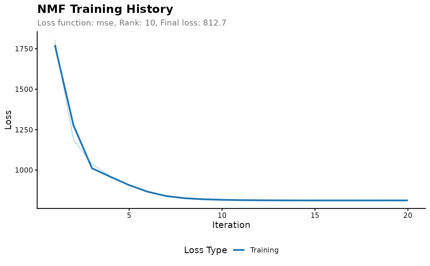
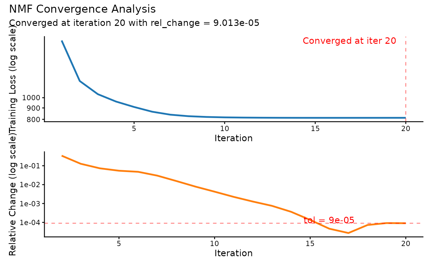
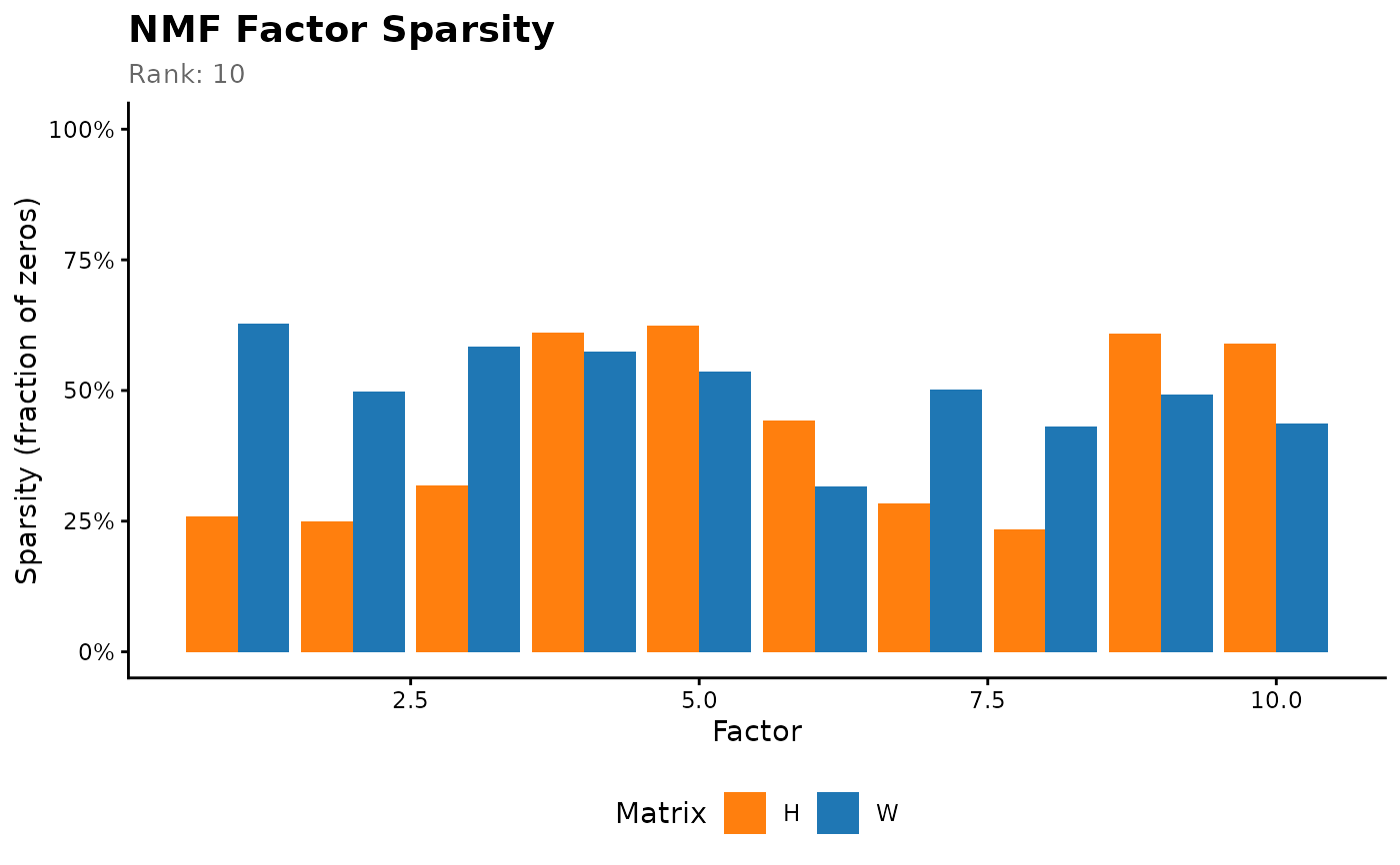
plot type: - "loss": Loss components over iterations (default) - "convergence": Log-scale loss convergence - "regularization": Regularization penalty contributions - "sparsity": Factor sparsity patterns

smooth

apply smoothing (LOESS) for noisy curves (default TRUE)

span

smoothing span for LOESS (default 0.3)

log_scale

use log scale for y-axis (default FALSE, auto TRUE for "convergence")

interactive

create interactive plotly plot (default FALSE)

theme

ggplot2 theme: "classic", "minimal", "dark" (default "classic")

...

additional arguments passed to specific plotting functions

Value

ggplot2 or plotly object

See also

nmf, compare_nmf

Examples

# \donttest{
# Basic loss plot
model <- nmf(hawaiibirds, k = 10)
plot(model)


# Convergence analysis
plot(model, type = "convergence")


# Interactive plot
plot(model, type = "loss", interactive = TRUE)


# Compare multiple runs
models <- replicate(5, nmf(hawaiibirds, k = 10), simplify = FALSE)
plot(models[[1]], type = "sparsity")

# }